Exercise 3: Motion Planning

In this exercise, you will explore motion planning between waypoints using polynomial trajectories. Given pre-planned path waypoints, your goal is to calculate minimum-jerk polynomial trajectories and make your drone navigate through a field of obstacles safely, smoothely and as fast as possible!

Task description

First, in Webots, open crazyflie_world-motion_planning.wbt and take a look at the obstacle map, it should look as shown in the Figure below.

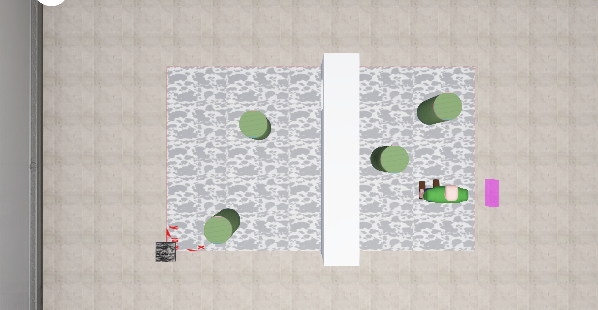
The map shows a take-off location, some obstacles and even a small gap through which you must plan a smooth path in order to reach your final goal. The final goal is indicated by a pink square.

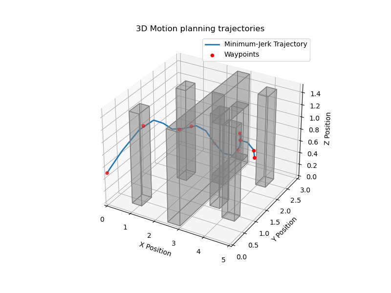
With exp_num = 3 in main.py, launch the simulation. You will see a waypoint map in a 3D environment, as shown below:

The red waypoints are sampled from a 3D A* path planner, giving you the shortest path with the fewest number of waypoints to reach the final goal while avoiding all obstacles which have been inflated by an additional 0.25 meters. However, A* assumes separate straight-line connections between the waypoints, such that your drone movements will not be smooth while following this path.

To improve smoothness and plan a feasible trajectory for the drone to follow, you will calculate polynomial trajectories that are continouous in velocity, acceleration, jerk and snap about every waypoint.

Exercise

Part 1 - Implementation

You will implement your code in the file ex3_motion_planner.py.

It is suggested to take the lecture slides as a reference for the motion planner implementation.

Go to the function compute_poly_matrix. This function defines a matrix A_m(t) such that \(x_m(t) = A_m(t)c_m\) at a given time t, where \(x_m(t) = [x, \dot{x}, \ddot{x}, \dddot{x}, \ddddot{x}]^T\) and the unknown polynomial coeffcients of a path segment are given as \(c_m = [c_{0,m}, c_{1,m}, c_{2,m}, c_{3,m}, c_{4,m}, c_{5,m}]^T\). This will later be used to define the constraint system of equations at every path segment.

By hand, calculate \(x_m(t) = [x, \dot{x}, \ddot{x}, \dddot{x}, \ddddot{x}]^T\) based on the given mimimum-jerk trajectory solution x(t) from the lecture.

From your solution, implement the variable A_m as a 2D 5 x 6 np.array in function of t such that it fulfills the system \(x_m(t) = A_m(t)c_m\).

Go to the function compute_poly_coefficients. This function takes in the A* waypoints path_waypoints in an array of dimension m. It solves the entire system of constraint equations \(A_{tot}c = b_{tot}\) to yield the polynomial coefficients \(c\) for all of the (m-1) path segments between the start and goal position.

Here, your task is to fill the 6(m-1) rows of the matrix \(A_{tot}\) and vector \(b_{tot}\) to contain all initial and final position, velocity and acceleration constraints as well as the continuity constraints for position, velocity, acceleration, jerk and snap between two consecutive path segments.

To help your implementation, you are given the vector seg_times, which contains the relative duration of each path segment as derived from self.times.

For each dimension in x,y and z direction, the matrix \(A_{tot}\) and vector \(b_{tot}\) and an array pos containing m waypoint positions for the respective dimension are already initialized.

For every dimension x, y, and z, iterate through the path segments to fill all 6*(m-1) rows of the matrix \(A_{tot}\) and the vector \(b_{tot}\) using the ion compute_poly_matrix to define initial, final and continuity constraints for each path segment (see the hint below for more)

Solve the system \(A_{tot}c = b_{tot}\) for every x,y and z dimension. The coefficent vector \(c\) for each dimension is then added to a 2D np.array poly_coeffs of dimensions (6(m-1) x 3).

Hints: Before you begin, check the uses of the function compute_poly_matrix provided in the function. The matrix A_0 is calculated as \(A_m(t=0)\) and is applicable for the initial conditions at every path segment. You can use this matrix to fill the the rows of \(A_{tot}\) with the initial constraints for velocity, acceleration and position. Similarly, A_f is calculated as \(A_m(t=\text{seg_times[i]})\) to describe the constraint matrix entries at the end of the i-th path segment. You can use this matrix to define your final constraints for velocity, acceleration and position. To define the continuity constraints for position, velocity, acceleration, snap and jerk between two consecutive path segments, you can use the matrices A_f and A_0 for the respective i-th and i+1-th path segment, filling the rows of \(A_{tot}\) such that \(x_{m,i}(t=\text{seg_times[i}])\) = \(x_{m,i+1}(t=0)\).

When all functions are implemented, run the simulation in Webots. You should see a trajectory plotted in blue at the start of the simulation (as per the figure below).

To validate your implementation, check the following: Does the trajectory pass through all of the red waypoints? Does the trajectory intersect any of the grey obstacles? Does the trajectory, on the whole, look continuous about the red waypoints?

When you are happy with your trajectory, close the plot and watch the simulation run. The drone should follow the trajectory and avoid the obstacles.

Note: If you receive an assertion error regarding the exceeding of the original velocity and acceleration limits, there are errors in your implementation.

Part 2 - Trajectory finetuning

Turn on the crazyflie camera overlay. It is possible that you see your drone moving in a rather jagged fashion between certain waypoints. This means that the polynomial trajectory should be discretized at smaller intervals to be used as a reference by the drone controller.

In the function init_params, the variable self.disc_steps can be used to tune this. Increase this value in small increments until you see smoother motion.

When your drone moves sufficiently smoothly and you obtain no collisions, study the vector self.times. Every entry in this vector corresponds to the predefined absolute time at which the drone should pass a corresponding waypoint.

Note: At the starting point, self.times[0] = 0. At the goal position the last entry self.times[m-1] corresponds to a final time t_f taken to fly all m trajectory segments.

You can now reduce the total time taken for your drone to reach the goal point by changing the variable t_f. At the start of every run, you will further see the maximum velocity and acceleration achieved during the run. Upon trajectory completion, the total time taken is displayed and should approximately coincide with the value of t_f.

If you obtain an assertion error that these values exceed the specified limits, increase self.vel_lim and self.acc_lim accordingly. How low can you set your time without crashing and upsetting the poor PhD student that is stuck in the drone dome :(?

(BONUS) The vector self.times is implemented such that every path segment should be completed within the same amount of time. However, depending on the length of each path segment, this may mean that in certain path segments your drone is constrained to accelerate faster if the path segment is long or slower if it is short.

Can you modify the vector self.times to yield a better distribution of times, such that the indicated average velocity and peak acceleration are lower? Can you achieve an even faster time to complete the run without crashing with your implementation?

(EXTRA BONUS) When flying aggresively, your drone may have some close calls with obstacles. This may be as the trajectory intersects the inflation zone about the obstacles. Can you implement a collision check and decoupled trajectory replanning step, as introdcued in the lecture, to ensure that this does not happen? You may use the attribute self.obstacles containing obstacle vertices and widths for each obstacle and modify the run_planner function to assist you.